Motivation

In collaboration with Jay Anderson and Ben Christensen, we designed this project for our Correlated Data Capstone course taught by Dr. Brianna Heggeseth.

To Brianna, we sincerely want to thank you for being an amazing, patient, and compassionate professor and working with us throughout all our various ups-and-downs in this course and in this project.

Introduction

Shadowed by a barbarous history of racial policing and state-sanctioned violence, the American opioid epidemic has been a crucible for relentless mass death and blistering chasms of racial inequity. Opioids are a broad class of strong painkillers which include medically prescribed drugs, heroin, and chemically synthesized opioids; examples include Morphine, Vicodin, OxyContin, Percocet, and Fentanyl. Since the late 1990s, opioid abuse rates have been sharply increasing, not being classified as a national public health emergency until 2017, with the relative popularity of specific opioid classes varying over time and place; experts have generally broken the epidemic into three epochs or waves (Disease Control 2021):

1. Widespread abuse of prescription opioids (1999-2010)
2. Widespread abuse of illicit heroin (2010-2013)
3. Widespread abuse of synthetic opioids (i.e. fentanyl) (2013-Present)

While multiple factors have been instrumental in the rise of opioid abuse, widespread medical prescription of opiates in the fist wave was critical in establishing the necessary preconditions for epidemic status today. The history of lax medical opiate prescription is, however, also entrenched in racist logics that have persisted since President Nixon’s ‘War on Drugs’ campaign. Namely, the ‘War on Drugs’ campaign was a carefully designed attack on Black and anti-War communities throughout the United States where key campaign designer and Nixon’s aide, John Ehrlichman, admitted:

We knew we couldn’t make it illegal to be either against the war or black, but by getting the public to associate the hippies with marijuana and blacks with heroin, and then criminalizing both heavily, we could disrupt those communities. We could arrest their leaders, raid their homes, break up their meetings, and vilify them night after night on the evening news. Did we know we were lying about the drugs? Of course we did. (2018)

These specifically targeted attacks have had longstanding effects on the racial dimensions of the opioid epidemic. Namely, the Opioid epidemic is considered a predominantly “White” public health issue [as White people accounted for 70-85% of all opioid overdoses between 1999 and 2016 (KFF 2021). The dramatic racial disparities in opioid overdose is widely considered to be a byproduct of the War on Drugs racialization of opioid abuse and its resultant influences on the systematic non-prescription of painkillers to Black and Latinx communities (Swift 2019). While multiple analytic approaches have clarified the risk factors of opioid overdose, measuring opioid abuse is a generally more difficult task due to implicit negative survivorship biases (i.e., the people who die from overdose are not all the people using opioids) and sweeping variations in data infrastructure and reporting practices. While multiple analyses have presented sufficient evidence suggesting strong geographic dimensions to opioid overdose, neighborhoods in Seattle, King County, Washington are relatively unique and insufficiently studied. The paucity of reports on Seattle is especially troubling when considering the high prevalence of opioid related deaths, accounting for 67% of all drug-related deaths between 2010-2017 and claiming more lives than car accidents— a leading cause of death nationwide— in 2017 (Division 2017; Alcohol Institute 2022). Further, due to the dramatic wealth disparities between economically disenfranchised neighborhoods and neighborhoods of workers at major commercial and tech companies, Seattle is a rich case study of neighborhood level geographies.

This project is, then, an attempt to understand and identify neighborhood disparities of opioid use throughout Seattle, King County, Washington and potential risk factors during the second wave of the epidemic. Specifically, we aim to model narcotic arrest counts throughout Seattle between 2010-2013 using spatial regression with geotagged SPD arrest records accessed via the Seattle Open Data Portal and census tract-level demographic information from the 2010, 2011, 2012, and 2013 American Community Surveys accessed via the Tidycensus package in R.

Data

Using narcotic arrest cases, we intend to model opioid use by proxy throughout Seattle, King County, Washington. We accessed our data from the Seattle Police Department’s (SPD) Records Management System where every arrest report filed in the city is uploaded. The data set runs from 2008 to the present, and lists general information about the cases, such as the report number, the date, the crime, and a jittered GPS coordinate. We grouped crimes by census tract and aggregated them up to that level so that we could look at the count of narcotics related crimes within neighborhoods. Importantly, narcotic arrests were reported by SPD in census tracts outside of Seattle’s borders. While, we could account for these cases, we ultimately decided to specify our data to specify the 137 census tracts within the city of Seattle’s borders. We specifically used:

• Longitude and Latitude: The relative location of the crime.
• Year: The Year that the crime occurred.
• Narcotic Crime Arrest Count: a variable we created that is a count of all of the Narcotic related arrests per year per census tract.

Using the Tidycensus R package (Walker and Herman 2021), we pulled demographic, geographic, and economic data across King County at the census tract level from the 2010, 2011, 2012, and 2013 American Community Surveys (ACS; N=397). The ACS is a long-form survey conducted by the U.S. Census Bureau that aims to continually track the economic, demographic, and social development of neighborhoods across the United States in a 12-month period. As such, this data is an aggregation of responses in each census tract which is necessarily different from other aggregation levels (e.g. census block, census group, SIP code tabulation areas, etc.); across aggregation levels, census tracts are typically preferred by geographers because sample sizes are relatively homogeneous between tracts and provides one of the most granular levels of data. In addition to census data, Tidycensus also provides associated shapefiles for each reported census tract. We also used the Tigris (Walker 2022) package to directly download the water and road TIGER/Line shapefiles from the Census website. As our project aims to model narcotic arrests per tract by broad structural factors we used multiple variables encoding the economic and demographic characteristics of each neighborhood. We specifically used:

• White: The percent of residents identifying as White in a defined census tract.
  • To scale this coefficients to be practically significant, we multiplied this variable by 5.
• Black: The percent of residents identifying as Black in a defined census tract.
  • To scale this coefficients to be practically significant, we multiplied this variable by 5.
• Latinx: The percent of residents identifying as Hispanic/Latinx in a defined census tract.
  • To scale this coefficients to be practically significant, we multiplied this variable by 5.
• Immigrant: The percent of residents who immigrated to the United States living in a defined census tract.
  • To scale this coefficients to be practically significant, we multiplied this variable by 5.
• Age: The average age of residents living in a defined census tract.
• Income: The median yearly income of residents living in a defined census tract.
  • To scale this coefficient to be practically significant, we divided this variable by 100.

While many of these covariates are necessarily collinear (i.e. percent White and Median Income), we chose these due to sufficient evidence suggesting their effects on outcomes. We also created two indicator variables for a census tract (GEOID: 53033008100; Outlier) that was at dramatically higher risk of arrest than every other census tract across the models and for census tracts whose population was above the 80th percentile (Metropolitan). While these indicator variables were implemented across all models for the sake of consistency, their addition was particular important for our non-spatial negative binomial count model since this naive model cannot account for spatial clustering.

Methods

There are specific statistical considerations when working with count data. First, because standard OLS models assumes that outcome variables are continuous and potentially negative, OLS is inappropriate when modeling narcotic arrest counts since they are necessarily $\geq$ 0. While the most well-known count regression model uses a Poisson likelihood distribution, Poisson regression imposes a very strict assumptions that the true mean and variance of count data is equal; in applied analyses, data very rarely fulfills this assumption, due to non-constant variance or ‘over dispersion’. Further, the high frequency of zeros in our narcotic arrest data grossly inflates the dispersion of our data and presents other statistical challenges. The below figure plots our observed narcotic arrest counts across each year in the 2nd wave.

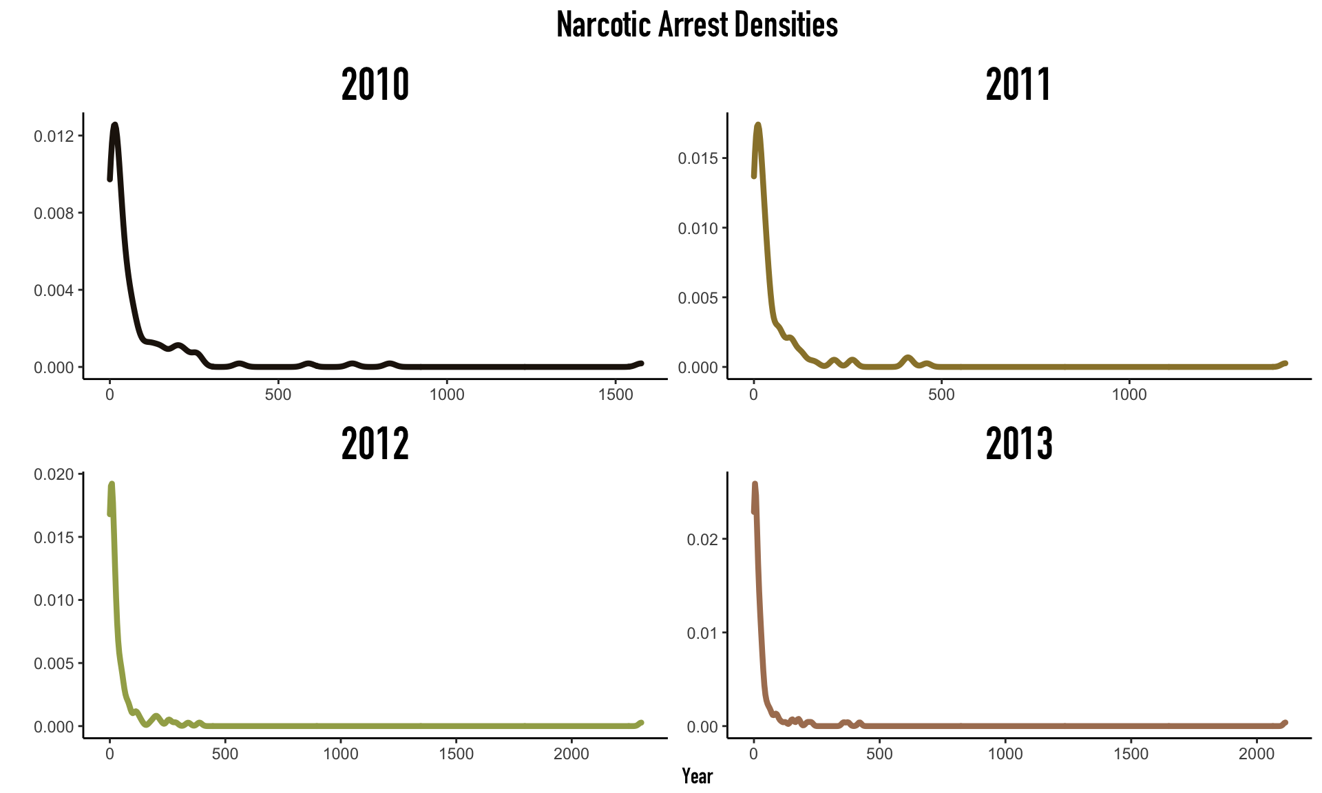
From the observed distributions, the clear zero-inflation and non-constant decay as count increases indicate that a simple poisson regression may be inappropriate. Although multiple approaches that account for zero-inflation exist, we performed standard negative binomial regression with a log-link function to model narcotic arrest counts for each year; we implemented this model to account for non-constant variance, establish crude baselines for comparison, and to motivate the application of spatial regression models since this technique cannot account for spatial clustering. Our four year-specific models of the arrest count in census tract, $i$, are of the form

$$Y_i \stackrel{iid}{\sim} NegBin(\mu_i, \mu_i +\frac{\mu_i}{k})$$ where $k$ is an estimated dispersion parameter and

$$ \begin{align*} \log(\mu_i) =& \beta_0 + \beta_1 \cdot \text{Outlier)}_i + \beta_2 \cdot \text{Metropolitan}_i+ \beta_3 \cdot \text{White}_i + \beta_4 \cdot \text{Income}_i +\\ &\beta_5 \cdot \text{Black}_i + \beta_6 \cdot \text{Age}_i + \beta_7 \cdot \text{Immigrant}_i + \beta_8 \cdot \text{Latinx}_i \end{align*}\\ $$

Once again, however, simple negative binomial regression cannot account for the underlying spatial relationships between observations that are nearby in space. As such, our predictions using the negative binomial model will be naive to the spatial connections between narcotic arrests. Specifically, our variance estimates will be biased and consequently lead to improper hypothesis tests. Luckily, there are various techniques which can account for the spatial correlation between observations.

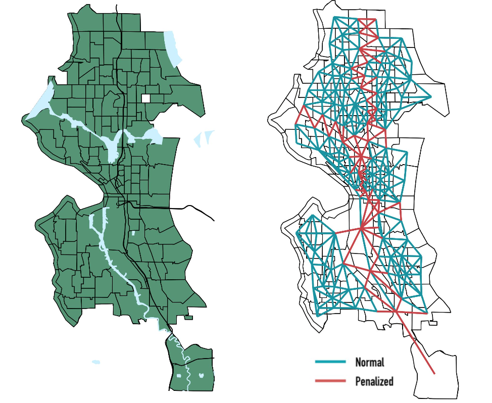
Neighborhood network structures (NNS) are formal mathematical objects that describe the connections between points or objects in space; they are especially critical in spatial data analysis so that we can encode how observations are correlated between each other in space. Considering a map, if two census tracts share a physical border (i.e. a whole line segment) or touch each other at a single point (i.e. a corner), a Queen NNS would state that these census tracts are ‘neighbors’ (i.e. they are similar to each other). Other neighborhood structures exist and are generally more conservative in their assessment of neighbor-status. For example, the Rook NNS would only consider census tracts that share a border ‘neighbors’, while a KNN structure would assign tracts neighbor-status according to their relative distances from one and other. We could further adjust any of these described NNS to adjust for the presence of substantial geographic/social barriers to produce penalized NNS that minimize the occurrence of tracts being naively-classified as neighbors, simply because they share a border. We computed a penalized Queen NNS for this analysis on narcotic arrest counts. We define our NNS below:

Let $W_{ij}$ be a $137\times 137$ weighting matrix of the $k$ census tracts in Seattle. If two census tracts, $i$ and $j$, share any border, then the entry at the $i$th row and $j$th column, $w_{ij}$, is set to 1; if the tracts don’t share a border, $w_{ij}$ is set to 0. Then, we first impose weighting constraints to account for the potential geographic separation of tracts, due to large bodies of water and major highways. If $i$ and $j$ are neighbors, but a major highway or body of water lies between them, then $w_{ij}$ is set to zero. Next, we set all entries along the diagonal to zero, as a tract can’t be its own neighbor. Finally, we weight the individual entries in a row, according to how many neighbors each census tract has, where every non-zero entry in a row are divided by the number of neighbors that census tract has, $k_{i}$. For example, if tract $\ell$ has 4 neighbors, then we divide all entries in the $\ell$th row by 4, and so all weights are set to 0.25. Following this weighting process, three tracts were removed because they were completely isolated by rivers and lakes and thus had no valid neighbors, leaving us a $134\times 134$ matrix. The below figure plots the observed Seattle census tracts waterways, and highways beside the proposed NNS.

The simultaneous autoregressive (SAR) model is a spatial regression technique that extends the standard regression frameworks to account for underlying spatial relationships between observations by weighting observations according to an underlying NNS (Whittle 1954; Hooten, Ver Hoef, and Hanks 2014; Wall 2004; Heggeseth 2022). The conditional autoregressive (CAR) model is another spatial regression technique that also adjusts for underlying spatial correlation between observations, but in a manner that is distinct from SAR models (Besag 1974; Wall 2004; Heggeseth 2022). Specifically, CAR models assume a Markov property or ‘memorylessness’ to the relationship between neighbors and thus impose weaker spatial correlation structures than SAR models (Wall 2004). The relative benefits of CAR and SAR models are highly contextual and specific to the data and problem at hand. Despite this difference, they do share the same general formula.

In this analysis, we implemented year-specific SAR and CAR models to predict average narcotic arrest counts within census tracts. We define our proposed models below:

$$\textbf{Y}=\lambda\boldsymbol{WY}+\boldsymbol{X\beta}+\boldsymbol{\epsilon}$$ where

• $Y$ is the vector of number of narcotic arrests for all $137$ census tracts.
• $\lambda\boldsymbol{WY}$ is a matrix product of some constant $\lambda$, our penalized proximity matrix $W$, and a matrix of narcotic arrests for all neighborhoods $Y$.
• $\boldsymbol{X\beta}$ is the product of the $134 \times 8$ covariate matrix— where entries of this matrix are the observed values of the $8$ predictors (columns) for the $134$ different census tracts (rows) in our data— and a $1 \times 8$ coefficient vector.
• $\boldsymbol{\epsilon}$ is the matrix of our tract-specific error terms with $\boldsymbol{\epsilon} \sim N(0,\sigma ^2I)$

Outside of this analysis, we performed model selection between our models, using standard evaluation metrics:

• Residual mapping and magnitude
• Bayesian Information Criterion (BIC) metrics
• Moran’s I Test Statistics of Residuals

Results

Exploratory Analysis

We aimed to model narcotic arrest counts throughout Seattle, King County, Washington using 3 separate candidate models. Prior to statistical analysis, we plot the observed incidence rates (IRs) for all 137 census tracts within the SPD patrol boundaries on the log scale.

| Year | Observed Incidence Rate | |:----: |:-----------------------: | | 2010 | 18.32843 | | 2011 | 12.86119 | | 2012 | 12.46315 | | 2013 | 10.42816 |

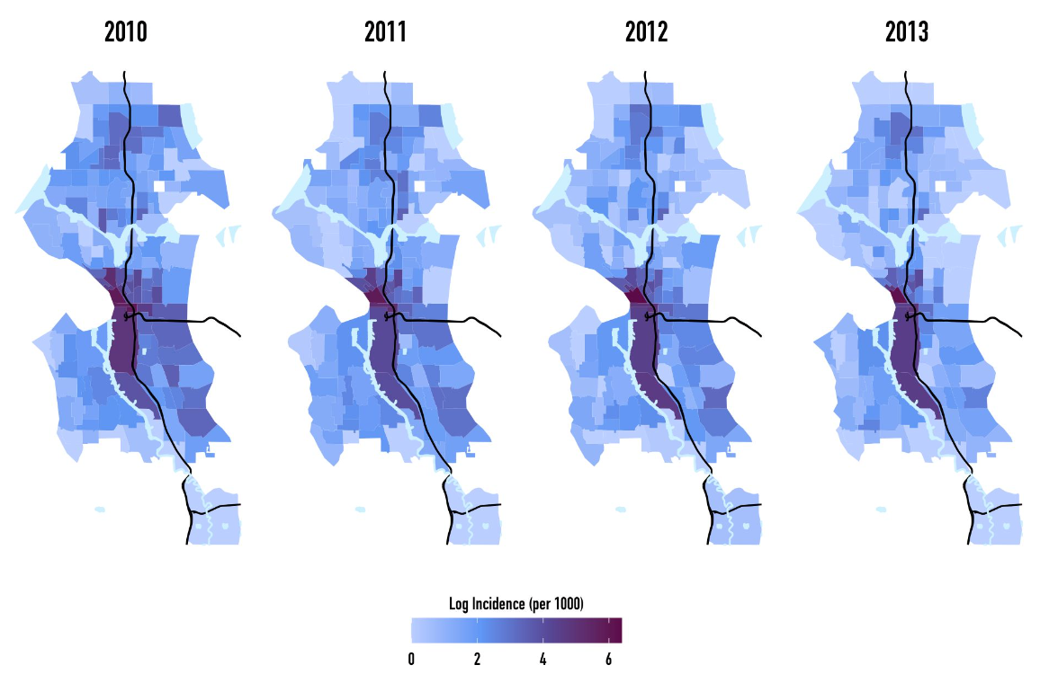
Yearly citywide IR estimates suggest that the incidence rate of narcotic arrests was highest in 2010 and lowest in 2013. However, the census tract counts narcotic arrests captured in the above figure demonstrate considerable spatial clustering of narcotic arrests between the I-5 and Duwamish Waterway in Seattle. Importantly, arrests were highly concentrated in Seattle’s Industrial and Downtown districts with the highest observed incidence rates occurring in one census tract (GEOID: 53033008100) encompassing Seattle’s Downtown district and Pioneer Square. Unlike the citywide estimates, these observed incidence rate estimates suggest that between 2010 and 2011, for every group of 1000 people, there would would be $\approx$ 358 narcotic-related arrests— a dramatic difference from the citywide estimate. Additionally, incidence rates in these metropolitan areas sharply increased in 2012 and 2013, with IR estimates of 592 in 2012 and 496 in 2013.

Next, we compare observed narcotic arrests IRs to the various demographic and economic variables we proposed to study: White, Black, Latinx, Immigrant, Age, and Income.

Like narcotic arrests, many of our proposed predictors demonstrate clear spatial clustering behaviors. Namely, the percent of white residents was negatively spatially associated with arrest incidence rates across all year, while immigrant percent was positively associated. However, due to demographic transitions across Seattle many of these associations may differ by year. Covariate maps demonstrate some slight collinear trends between average age and income where the wealthiest census tracts also tended to be some of the oldest. While income was negatively associated with both Black, Immigrant, and Latinx percentages.

Model Comparison

Using three candidate models stratified by year, we aimed to study narcotic arrest counts by census tracts in Seattle, King County, Washington. This section outlines our model selection process, using residual mapping, Bayesian Information Criterion (BIC) metrics, and spatial Moran’s I residual tests for each of the three model types across all four years.

**Simple Negative Binomial (with and without outliers)** **Simultaneous Autoregressive Model** **Conditional Autoregressive Model** | Year | Negative Binomial | SAR | CAR | |:----: |:-----------------: |:---------: |:--------: | | 2010 | 11.43584 | 15.553052 | 14.99905 | | 2011 | 13.73855 | 18.710910 | 19.53239 | | 2012 | 45.55720 | 9.956018 | 14.71446 | | 2013 | 116.89098 | 9.677963 | 12.54004 |

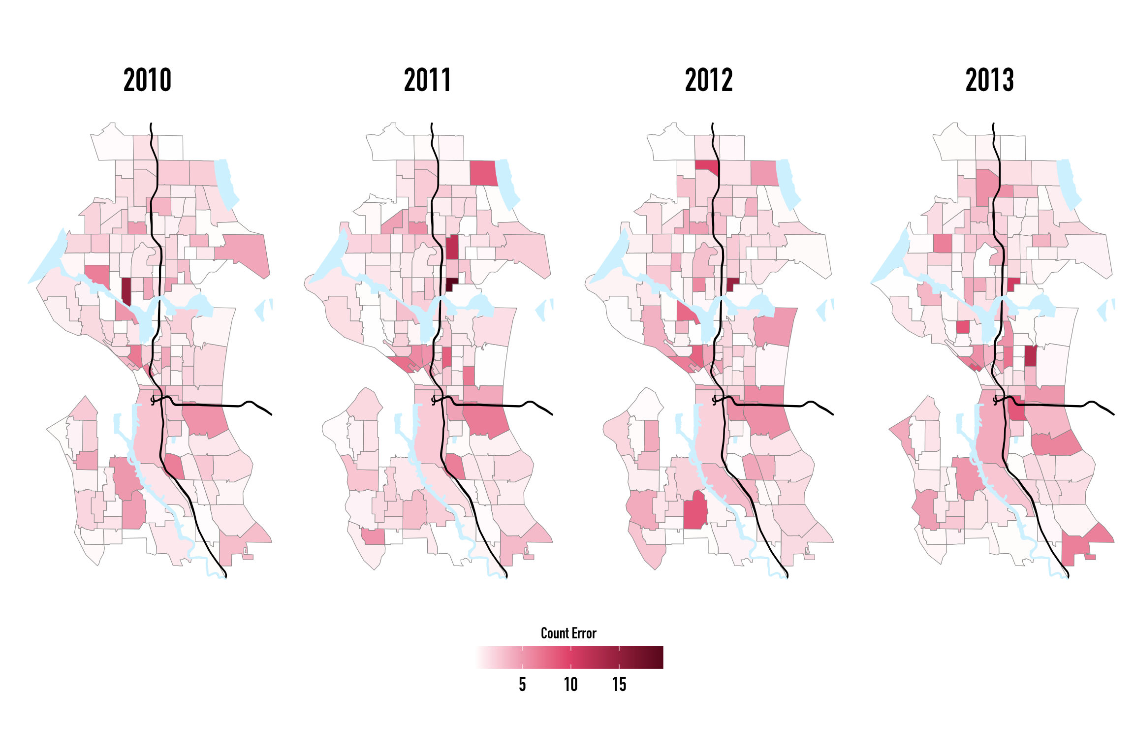
Spatial trends in the negative binomial residuals were largely obscured by the presence of one census tract that we grossly mispredicted by $\approx$ 117 counts. After removing this tract from our visualization, there was ostensible spatial clustering in tracts centered at the intersection of 1-5 and I-90 highways, in the Downtown districts, and in the Industrial districts besides the Duwamish waterway. Further, it seemed that our model’s predictions of census tract arrest counts performed worst in 2013.

In contrast, the magnitude of our SAR and CAR model residuals were dramatically smaller magnitude for every year and far more randomly distributed across census tracts, exhibiting no clear spatial clustering patterns. Considering the magnitude of our residual errors, the SAR and CAR model residuals were largely comparable in the beginning years of the second opioid epidemic wave (2010-2011), but in the later years the SAR model had the smallest count errors for all models— mispredicting arrest by at most 9 counts.

Across spatial models and year, one census tract was systematically mispredicted. On the North Western edge of the University of Washington campus, the section of the University district was the most inaccurately predicted tract with CAR model residuals more than 2x greater than the error of the next closest tract.

Moran’s I

The Moran’s I Test is a statistical test used to identify the occurrence of spatial clustering via standard hypothesis testing where the null, $H_0$, assumes that residuals are independent over space. In this analysis, we use the Moran’s I hypothesis test on our residual errors to identify if there is leftover spatial effects on our model. In this section, we present tables of our Moran’s I test output for each of our three models over time.

Below is the Moran’s I test output on our negative binomial residuals.

| Year | p-value | Moran I statistic | Expectation | Variance | |:-----: |:--------: |:-----------------: |:-----------: |:---------: | | 2010 | 0.00e+00 | 0.3135200 | -0.0075758 | 0.0026623 | | 2011 | 7.00e-07 | 0.2481396 | -0.0075758 | 0.0026553 | | 2012 | 8.40e-06 | 0.2208913 | -0.0075758 | 0.0026315 | | 2013 | 1.99e-05 | 0.2093290 | -0.0075758 | 0.0025846 |

From the above table, we found statistically significant evidence of positive spatial correlation (Moran I statistic > 0) in our residual errors for every year in our study (p-value < 0.05), suggesting that nearby errors are correlated. As such, we reject $H_0$ and conclude that our simple negative binomial model could not sufficiently model narcotic arrests because arrests are spatially correlated. Interestingly, the magnitude of spatial clustering (Moran I statistics) varied over time with 2010 seeing the highest clustering and 2012 seeing the lowest.

To account for the identified spatial clustering, we performed the same hypothesis test on our SAR and CAR model residuals and verify their utility for modeling narcotic arrests. Below, are our Moran’s I test results for the SAR model.

| Year | p-value | Moran I statistic | Expectation | Variance | |:-----: |:---------: |:-----------------: |:-----------: |:---------: | | 2010 | 0.5213880 | 0.0254418 | -0.0075758 | 0.0026515 | | 2011 | 0.4052197 | 0.0352947 | -0.0075758 | 0.0026529 | | 2012 | 0.4737983 | 0.0294463 | -0.0075758 | 0.0026713 | | 2013 | 0.3782288 | 0.0380083 | -0.0075758 | 0.0026762 |

Using a SAR model structure, we found insufficient evidence to reject the $H_0$ and ultimately the absence of spatial correlation between observations across all years (p-value > 0.05). This is good! This means that our SAR model sufficiently accounted for the spatial autocorrelation between narcotic arrests and can then produce reliable hypothesis tests.

| Year | p-value | Moran I statistic | Expectation | Variance | |:-----: |:---------: |:-----------------: |:-----------: |:---------: | | 2010 | 0.0143041 | -0.1339276 | -0.0075758 | 0.0026607 | | 2011 | 0.1599391 | -0.0800319 | -0.0075758 | 0.0026584 | | 2012 | 0.0167360 | -0.1312093 | -0.0075758 | 0.0026704 | | 2013 | 0.1781474 | -0.0772408 | -0.0075758 | 0.0026769 |

From the above table, we found statistically significant evidence of positive spatial correlation (Moran I statistic > 0) in our residual errors for 2010 (p-value = 0.014) and 2012 (p-value = 0.016). As such, we reject $H_0$ and conclude that our CAR model could not sufficiently model narcotic arrests because arrests are spatially correlated.

BIC

The Bayesian Information Criterion (BIC) is a model selection technique that penalizes overfit models by implementing penalty terms for the number of parameters in a given model. Here, we use BIC computations to compare our three models and select the model with the lowest BIC metrics. The following table presents the BIC values for the negative binomial, SAR, and CAR models across our four year time period.

| Year | Negative Binomial | SAR | CAR | |:----: |:-----------------: |:--------: |:--------: | | 2010 | 1381.217 | 459.2198 | 474.4112 | | 2011 | 1292.076 | 489.8557 | 499.3556 | | 2012 | 1239.588 | 502.6637 | 509.9817 | | 2013 | 1177.707 | 488.0485 | 497.4415 |

Across all three models, the SAR model consistently had the best BIC metrics for all years in our study. Although the negative binomial and SAR BICs were dramatically different, the differences between SAR and CAR models were marginal. For both spatial models, there was meaningful temporal variation in BIC estimates, with both spatial models performing best in 2010 and worst in 2012. While the negative binomial model never outperformed the SAR or CAR models, negative binomial BIC metrics were worst in 2010 and best in 2013. As indicated by our Moran’s I test, there is some considerable variation in the spatial effects over time which may be reflected in the temporal shifts in these BIC metrics.

Final Analytic Model

Across all three categories and throughout time, our SAR model greatly outperformed the other candidate models. Specifically, due to small residual magnitudes, the absence of residual spatial clustering, and generally good BIC metrics, we will use our finalized SAR model to predict narcotic arrests in throughout Seattle.

Using our SAR model with $\alpha=0.05$ and when controlling for other covariates, we found sufficient evidence to conclude that major metropolitan areas (i.e. total population above the 80th percentile) had statistically significant elevated risks of narcotic arrests relative to all other census tracts, regardless of the year. However, most other predictors had time-varyingly significant effects on the risk of narcotic arrests; for the sake of brevity, we exclusively list the significant predictors for each year-specific SAR model in the following tables.

term	estimate	std.error	z.value	p.value
majorTRUE	94.85268	0.2363774	2.822070	0.0047715
black	216.64634	0.4527111	2.546028	0.0108956
immigrant	134.38144	0.3977942	2.141257	0.0322533

| term | estimate | std.error | z.value | p.value | |:---------: |:---------: |:---------: |:--------: |:---------: | | majorTRUE | 114.2626 | 0.2619126 | 2.909489 | 0.0036202 | | white | 4800.3169 | 1.7940684 | 2.169307 | 0.0300594 | | black | 263.6595 | 0.4627853 | 2.789734 | 0.0052751 | | immigrant | 210.1960 | 0.4537137 | 2.495041 | 0.0125943 | | term | estimate | std.error | z.value | p.value | |:---------: |:--------: |:---------: |:--------: |:---------: | | majorTRUE | 153.9560 | 0.2796861 | 3.332274 | 0.0008614 | | latinx | 244.0459 | 0.4765524 | 2.592799 | 0.0095198 | | term | estimate | std.error | z.value | p.value | |:----------: |:-----------: |:---------: |:---------: |:---------: | | excessTRUE | 920.40565 | 1.0810157 | 2.148706 | 0.0316577 | | majorTRUE | 114.45400 | 0.2453656 | 3.109340 | 0.0018751 | | white | 18694.91763 | 1.7932750 | 2.919893 | 0.0035015 | | med_income | -99.18991 | 1.3696090 | -3.516174 | 0.0004378 | | immigrant | 374.84528 | 0.4590921 | 3.393260 | 0.0006907 |

From the tables it’s clear that there were meaningful temporal trends in the significance and effects of predictors on narcotic arrests. For example, in 2010 5% increases in Black and Immigrant residents were associated with 216% and 134% increases in the risk of narcotics arrest, but neither were significant predictors of arrests in 2012. Likewise, 5% increases in White residents were associated with profoundly elevated risks of arrest in 2011 and 2013 (2011: 4800% and 18694%). Surprisingly, a tract’s median income was only statistically significantly related to risk of arrest in 2013— exhibiting a negative relationship with risk of arrest. Likewise, only in 2013 was our outlier census tract at elevated risk of arrest relative to all other census tracts, claiming a 920% increase in the risk of arrest.

Conclusions

Using narcotic arrest counts reported by the Seattle Police Department from 2010 until 2013, we aimed to identify neighborhood disparities in the risk of drug/narcotic related arrests as a proxy for opioid abuse and characterize the roles that neighborhoods played in the second wave of the Opioid epidemic. Specifically, using simultaneous autoregressive (SAR) models with penalized Queen structures, we modeled narcotic arrests according to multiple economic and demographic variables. We found dramatic disparities in the risk of narcotic-related arrests between neighborhoods that show unique changes in which racial demographics may have been at risk of arrest at various points across time. Generally, we found that densely populated census tracts were at significantly elevated risks of narcotic arrests, regardless of the year. However, we found temporal trends in the statistical significance of all other predictors, likely due to the demographic transitions of narcotic abuse within Seattle. Although model estimates suggest that increasing proportions of Black, Latinx, and Immigrant residents were all associated with elevated risks of arrest, increasing proportions of White residents were uniformly the highest risk factors of narcotic arrests, with 5% increases in White proportion associated with 48x and 187x elevated risks of arrest in 2011 and 2013. It is entirely plausible that the large magnitude of these associations may reflect the known racial disparities in opioid abuse which paint opioid abuse as a predominantly White issue. To our surprise, we found that median income was not statistically significantly related to the risk of arrest for all years except 2013 where it had a negative association with risk of arrest. The non-significance of income in the early years of narcotic arrest is interesting, given that studies have suggested that low socioeconomic status is strongly associated with opioid overdose (Altekruse et al. 2020). While these non-significant relationships in the early years of the epidemic could be due to the arrests of people that are not typically surveyed by the census (i.e. unhoused populations, undocumented immigrants, etcetera), it is unclear why socioeconomic status was not a key risk factor in risk of arrest.

Arrest count mapping showed evidence of strong spatial clustering that is mainly centralized in the Downtown, Pioneer Square, and the Industrial District neighborhoods. The strong clusterings may be due to multiple factors. As Seattle’s economic center, it is plausible that these areas are the most heavily policed neighborhoods in Seattle and thus have inflated arrest counts by virtue of increased patrolling— not elevated narcotic use. Not only could there be more police patrolling these neighborhoods, but it’s plausible that the unhoused populations of Seattle— a group historically victimized by the police and disproportionately affected by the opioid crisis— may live or often congregate in these neighborhoods. Additionally, racist and machiavellian police practices— such as racial profiling, false arrests, and arrest quotas— may further bias arrest counts if predominantly non-White neighborhoods are policed at higher rates. Given the racial dimensions of the opioid epidemic and the role the War on Drugs had on percolating current narcotic policing practices, the elevated risks of arrest for predominantly non-White neighborhoods— a trend that is in conflict with studies on the racial disparities in opioid abuse— may be an artifact of such racist policing practices.

Our study is, however, not without limitations. First and foremost, we should note that SPD’s narcotic arrest classifications are far broader and may provide an inappropriate proxy to measure opioid abuse. While performing spatial analysis using data collected from people diagnosed with opioid use disorder or non-fatal overdose would more accurately measure the scale of opioid abuse— as opposed to lethal overdose— necessary hospital data is not publicly available and firmly protected. As such, narcotic arrest data is sufficient in this context. Further, our models were uniformly weak at predicting narcotic arrest rates in a tract near the University District (GEOID: 53033005301), due to the simultaneously high proportion of young, wealthy, students and very high narcotic arrest rates. The combination of a very unique demographic make-up combined with the observed arrest numbers is a very plausible explanation for our models’ relatively poor performance. Lastly, a major limitation of our penalized Queen structure is that we needed to exclude three “isolate” census tracts because they had no neighbors under our proposed weighting structure. However, of these three tracts, the census tract near Union Lake was the only tract of interest, since the other two tracts were outside the official Seattle city limits and a non-residential harbor used for shipping. However, it is unfortunate that this weighting structure isolated South Union Lake— a tract of about 3000 total people and around 18 narcotic arrests per year— from all other census tracts in the Eastlake and Cascade neighborhoods. And given the opioid epidemic’s disproportionate impact on unhoused populations, our use of census data is also a very strong limitation of our study since these groups are exempt from the census and data collection on unhoused populations is generally scant.

References

2018. To Acknowledge That the War on Drugs Has Been a Failed Policy in Achieving the Goal of Reducing Drug Use, and for the House of Representatives to Apologize to the Individuals and Communities That Were Victimized by This Policy. https://www.govinfo.gov/content/pkg/BILLS-115hres933ih/html/BILLS-115hres933ih.htm.

Alcohol Institute, Addictions Drugs &. 2022. “Opioid Trends Across Washington State.” Washington State Opioid Trends. University of Washington. https://adai.washington.edu/WAdata/opiate_home.htm.

Altekruse, Sean F, Candace M Cosgrove, William C Altekruse, Richard A Jenkins, and Carlos Blanco. 2020. “Socioeconomic Risk Factors for Fatal Opioid Overdoses in the United States: Findings from the Mortality Disparities in American Communities Study (MDAC).” PLoS One 15 (1): e0227966. Besag, Julian. 1974. “Spatial Interaction and the Statistical Analysis of Lattice Systems.” Journal of the Royal Statistical Society: Series B (Methodological) 36 (2): 192–225. Disease Control, Centers for. 2021. “Drug Overdose.” Centers for Disease Control and Prevention. Centers for Disease Control; Prevention. https://www.cdc.gov/drugoverdose/epidemic/index.html.

Division, Seattle Field. 2017. Opioid Overdose Deaths Remain High in Seattle and King County. Heggeseth, Brianna. 2022. “7.4 Areal Data.” In Correlated Data Notes.

Hooten, Mevin B, Jay M Ver Hoef, and Ephraim M Hanks. 2014. “Simultaneous Autoregressive (SAR) Model.” Wiley StatsRef: Statistics Reference Online, 1–10. KFF. 2021. “Opioid Overdose Deaths by Race/Ethnicity.” KFF. Kaiser Family Foundation. https://www.kff.org/other/state-indicator/opioid-overdose-deaths-by-raceethnicity/?dataView=1¤tTimeframe=20&amp;selectedRows=.

Swift, M. Maria AND Elfassy, Samuel L. AND Glymour. 2019. “Racial Discrimination in Medical Care Settings and Opioid Pain Reliever Misuse in a u.s. Cohort: 1992 to 2015.” PLOS ONE 14 (12): 1–12. https://doi.org/10.1371/journal.pone.0226490.

Walker, Kyle. 2022. Tigris: Load Census TIGER/Line Shapefiles. https://CRAN.R-project.org/package=tigris.

Walker, Kyle, and Matt Herman. 2021. Tidycensus: Load US Census Boundary and Attribute Data as ’Tidyverse’ and ’Sf’-Ready Data Frames. https://CRAN.R-project.org/package=tidycensus.

Wall, Melanie M. 2004. “A Close Look at the Spatial Structure Implied by the CAR and SAR Models.” Journal of Statistical Planning and Inference 121 (2): 311–24. Whittle, Peter. 1954. “On Stationary Processes in the Plane.” Biometrika, 434–49.

R Packages

Alboukadel Kassambara (2020). ggpubr: ‘ggplot2’ Based Publication Ready Plots. R package version 0.4.0. https://CRAN.R-project.org/package=ggpubr

Bivand, Roger S. and Wong, David W. S. (2018) Comparing implementations of global and local indicators of spatial association TEST, 27(3), 716-748. URL https://doi.org/10.1007/s11749-018-0599-x

Garrett Grolemund, Hadley Wickham (2011). Dates and Times Made Easy with lubridate. Journal of Statistical Software, 40(3), 1-25. URL https://www.jstatsoft.org/v40/i03/.

Hao Zhu (2021). kableExtra: Construct Complex Table with ‘kable’ and Pipe Syntax. R package version 1.3.4. https://CRAN.R-project.org/package=kableExtra

Kirill Müller (2020). here: A Simpler Way to Find Your Files. R package version 1.0.1. https://CRAN.R-project.org/package=here

Kyle Walker (2021). tigris: Load Census TIGER/Line Shapefiles. R package version 1.5. https://CRAN.R-project.org/package=tigris

Kyle Walker and Matt Herman (2021). tidycensus: Load US Census Boundary and Attribute Data as ‘tidyverse’ and ‘sf’-Ready Data Frames. R package version 1.1. https://CRAN.R-project.org/package=tidycensus

Pebesma, E., 2018. Simple Features for R: Standardized Support for Spatial Vector Data. The R Journal 10 (1), 439-446, https://doi.org/10.32614/RJ-2018-009

Roger S. Bivand, Edzer Pebesma, Virgilio Gomez-Rubio, 2013. Applied spatial data analysis with R, Second edition. Springer, NY. https://asdar-book.org/

Sam Firke (2021). janitor: Simple Tools for Examining and Cleaning Dirty Data. R package version 2.1.0. https://CRAN.R-project.org/package=janitor

Stefan Milton Bache and Hadley Wickham (2020). magrittr: A Forward-Pipe Operator for R. R package version 2.0.1. https://CRAN.R-project.org/package=magrittr

Venables, W. N. & Ripley, B. D. (2002) Modern Applied Statistics with S. Fourth Edition. Springer, New York. ISBN 0-387-95457-0

Wickham et al., (2019). Welcome to the tidyverse. Journal of Open Source Software, 4(43), 1686, https://doi.org/10.21105/joss.01686

Winston Chang (2012). extrafontdb: Package for holding the database for the extrafont package. R package version 1.0. https://CRAN.R-project.org/package=extrafontdb

Winston Chang, (2014). extrafont: Tools for using fonts. R package version 0.17. https://CRAN.R-project.org/package=extrafont